15-618 Final Project
Final Report
Parallelizing Betweenness Centrality on CPU and GPU
Summary
We implemented Brandes' Betweenness Centrality on two parallel
platforms, a multi-core CPU using OpenMP and an NVIDIA RTX 2080
using CUDA. The CPU implementation parallelizes the outer source
loop and reaches up to 7.36× speedup at 8 threads through
thread-local accumulation, and supports a sampled mode that
handles large scale graphs (web-Google at 916,428
vertices) at predictable runtime. The GPU side worked through a
profiling-driven sequence of three within-source optimizations
that each addressed one bottleneck but worsened another, before
pivoting to a multi-source design that runs many BFS computations
side by side and dominates every within-source attempt. At 32
sources the multi-source GPU design is the fastest implementation
on every graph we measured. At full source count the GPU wins on
the larger and denser real graphs while OpenMP wins on the smaller
graphs whose working set fits in L3 cache.
Background
Betweenness Centrality
Betweenness Centrality (BC) measures the importance of a vertex in a graph by the fraction of shortest paths that pass through it. For a graph G = (V, E), the BC score of a vertex is the sum across all source-target pairs of the ratio of shortest paths from s to t that go through v divided by the total number of shortest paths from s to t. A node with high BC sits on many shortest paths and controls a lot of information flow. Naive computation needs all-pairs shortest paths and runs in O(V3). Brandes' algorithm reduces this to O(VE).
Brandes' Algorithm
Brandes runs the same BFS plus dependency walk once per source vertex. For each source, the forward BFS records the shortest path distance and the number of shortest paths to every reachable vertex. The backward dependency pass walks visited vertices in reverse depth order and accumulates each vertex's contribution into the global BC array.
The outer loop over sources is fully data-parallel because the iterations have no shared dependencies, and is the natural target for parallelism. Within a single source, the BFS must run in level order, but each level itself can be expanded in parallel.
Graph Representation
Both CPU and GPU implementations use Compressed Sparse Row (CSR) format. Each input edge is treated as undirected and stored as two directed CSR entries. This doubles the edge count relative to the raw input but keeps traversal consistent across all datasets.
Datasets
We evaluate on six SNAP graphs of varying structure
(line_10000, ca-GrQc,
p2p-Gnutella04, wiki-Vote,
ego-facebook, soc-Slashdot0811) plus
web-Google (916,428 vertices) for the sampled
approximation experiments. The first six are used for exact BC.
web-Google is too large for exact all-source BC in a
reasonable time budget.
Each visualization below shows the top 100 highest-BC vertices for one dataset. Node size and color are proportional to the BC score.
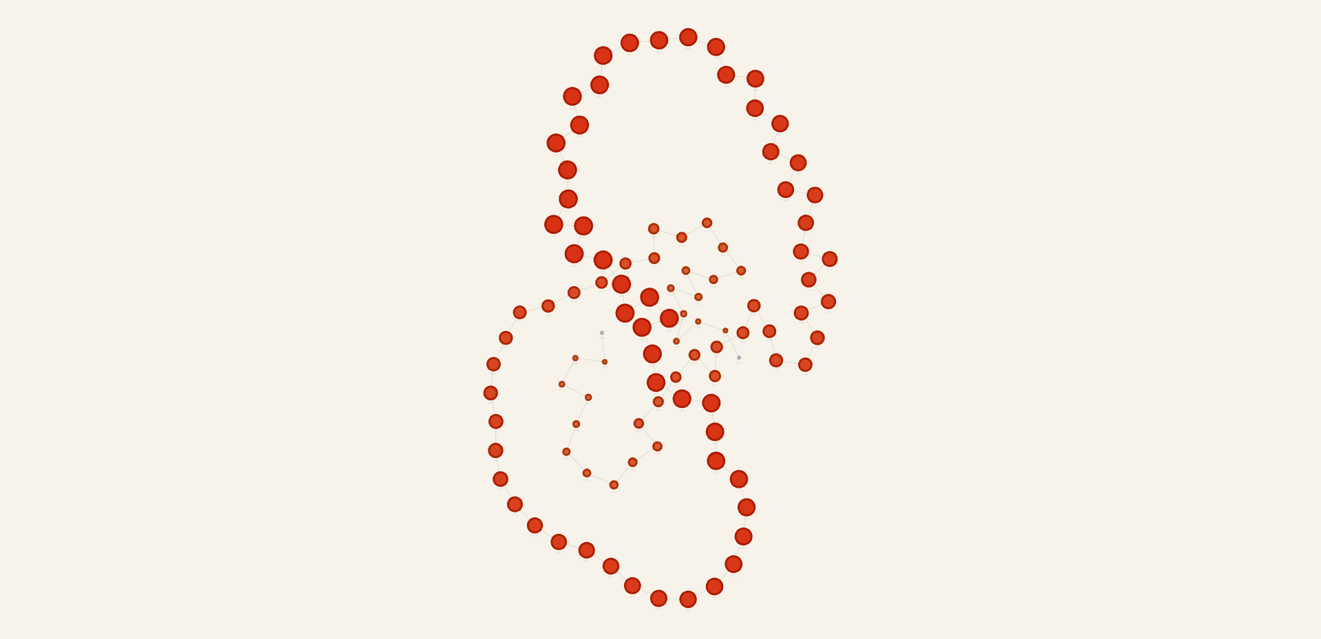
line_10000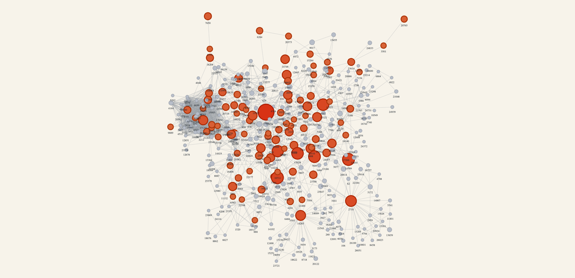
ca-GrQc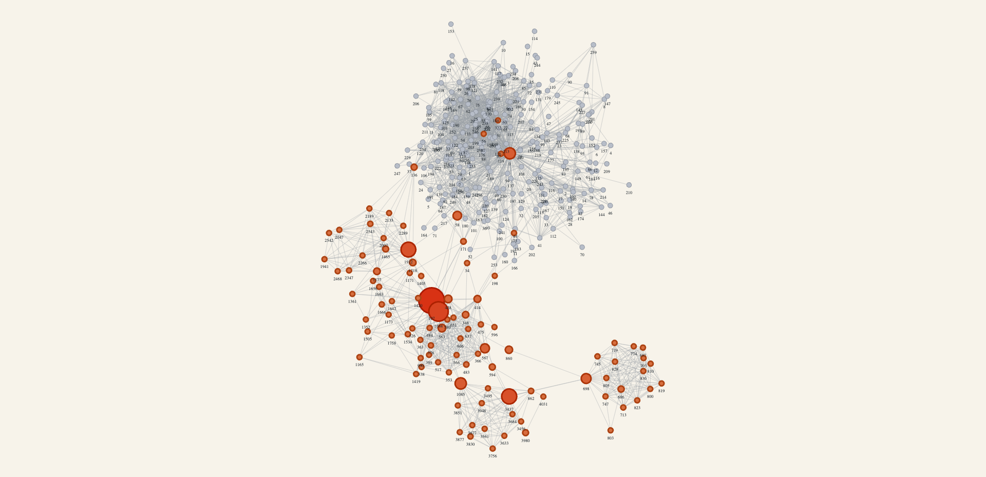
ego-facebook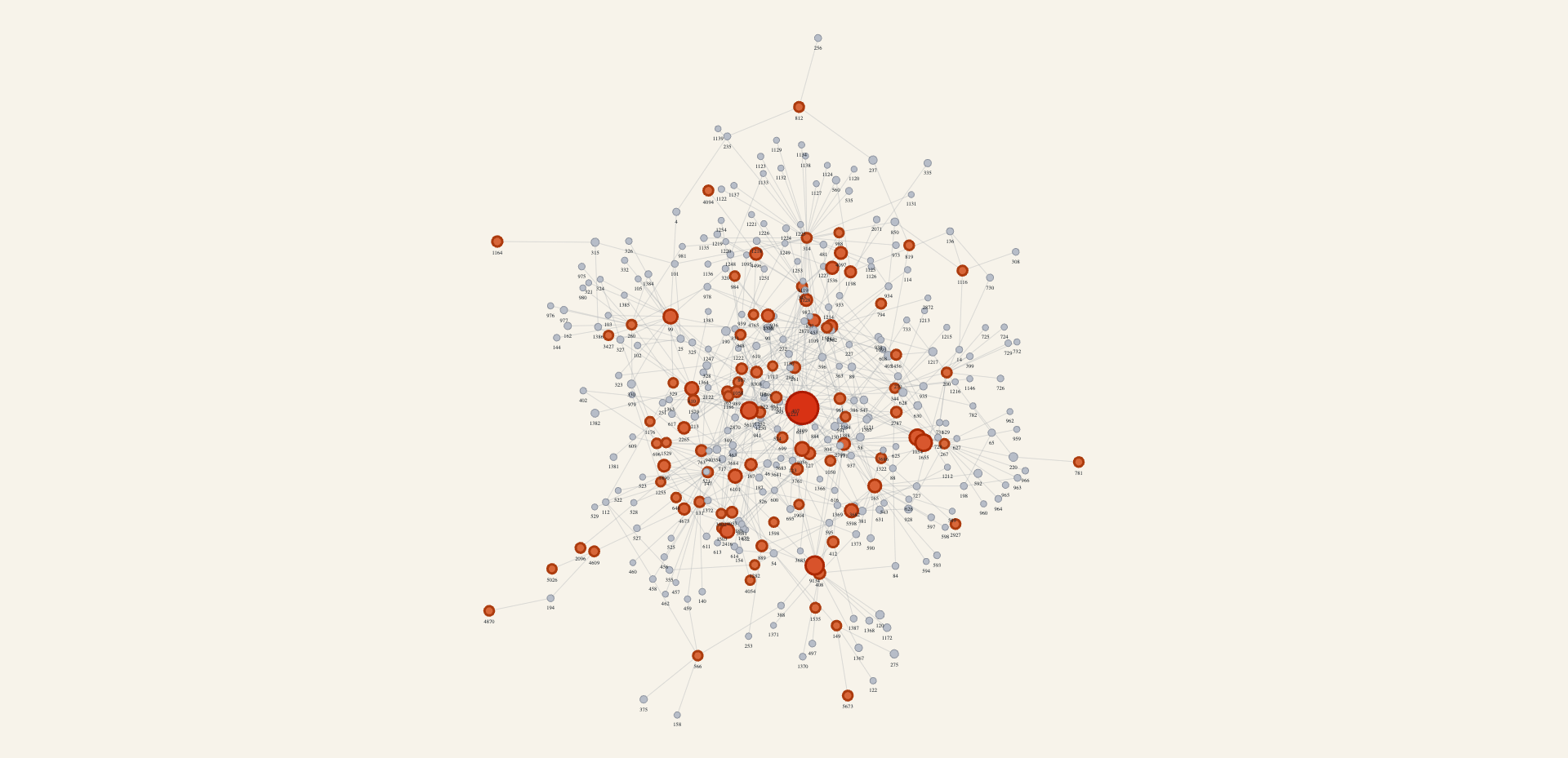
p2p-Gnutella04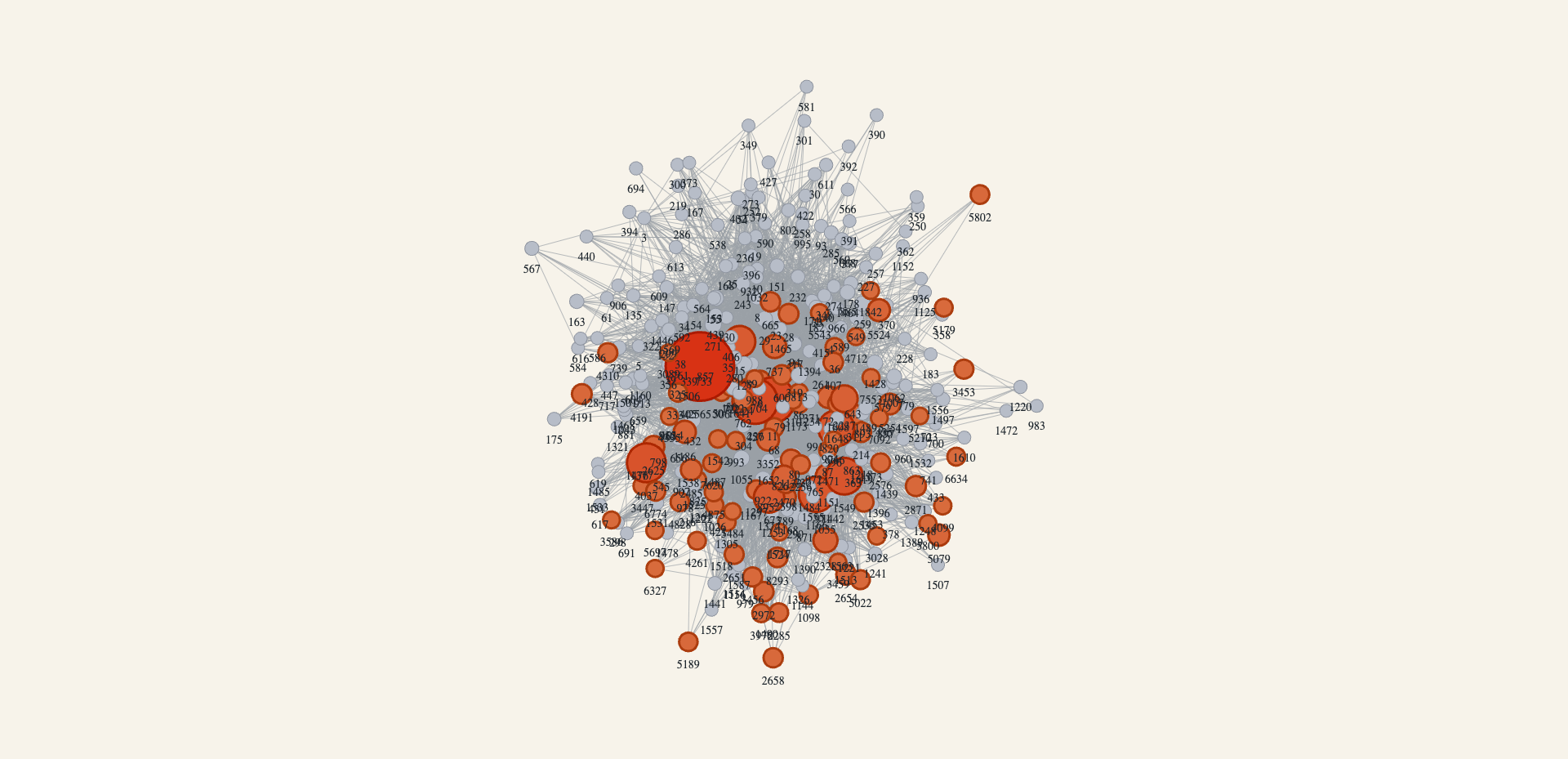
wiki-Vote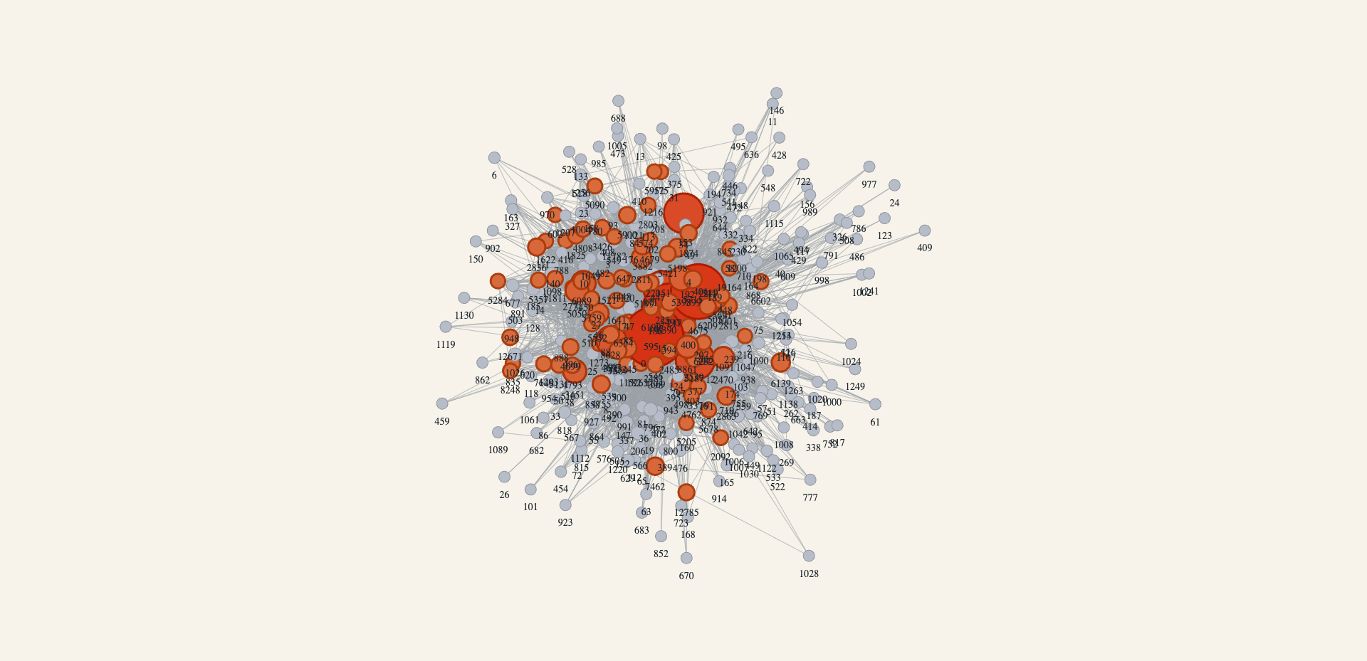
soc-Slashdot0811Approach
The project has two parallel tracks, CPU with OpenMP and GPU with CUDA, both benchmarked on the GHC 28 machine.
CPU Track
The serial implementation is a direct C++ realization of Brandes' algorithm and is the correctness oracle that every other implementation in the project is checked against. The first OpenMP attempt parallelized the outer source loop with a shared thread-by-vertex BC array, then merged the array column-wise at the end. The merge dominated runtime because the layout was cache-unfriendly.
The redesign moved to per-thread local accumulation. Each thread keeps a private BC array as it processes its assigned sources, and merges that local array into the global result exactly once at the end. Synchronization stays out of the hot path and the cache-hostile reduction disappears.
For graphs that are too large for exact all-source Brandes, the
CPU implementation supports a sampled mode. It
picks a deterministic subset of source vertices, runs Brandes
from each, and scales the result by the ratio of total to
sampled. This is the only mode we use on
web-Google.
GPU Track
Brandes has two axes of parallelism, an outer loop over sources
and an inner BFS level. Earlier GPU versions used only the inner
level, which left most SMs idle whenever the active vertex set
was small. The final implementation uses both at once with a 2D
launch grid where each thread is a (vertex, source) pair, and
the per-source state is laid out source-major as [s * V +
v] so consecutive lanes in a warp read consecutive memory
and coalesce into one transaction.
Three Bottlenecks Identified by Nsight
- Hub vertex contention. Memory stalls dominated the warp-cycle breakdown. Many edges into the same high-degree hub serialize on atomic updates and the rest of each warp sits idle waiting its turn.
- Idle threads. The scheduler was eligible to issue a warp on only ~3% of cycles. Most threads belonged to edges whose source vertex was not at the current depth, so they read, discarded, and exited.
-
Host-device sync overhead. One synchronization
plus one PCIe transfer per BFS level. On
line_10000with 32 sources times 9,999 levels, that is 319,968 transfers, each pausing the GPU for tens of microseconds.
Three Within-Source Attempts
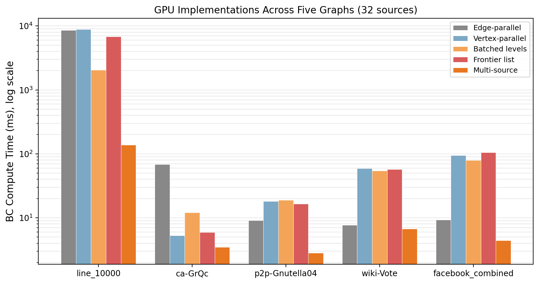
- Vertex-parallel BFS (targets bottleneck 2). Switched from one thread per edge to one thread per vertex. Wins 12.9× on sparse graphs but regresses 10.2× on dense ones because hubs become single-threaded sequential walks.
- Batched level execution (targets bottleneck 3). Launch 32 BFS levels in a row in the same CUDA stream, then sync once. CUDA preserves stream order. Recovers a large fraction of lost time on the chain graph but does not help on social graphs.
- Active-vertex queue (targets bottleneck 2 more aggressively). Maintain an explicit list of currently-active vertices each level. The host has to read the list size every level, which re-introduces the synchronization pattern attempt 2 had eliminated.
Lesson. No single within-source design was best on every graph. Each addressed one bottleneck but revealed another. A single source's BFS at a given depth only has so much parallelism in it.
Multi-Source Optimization
We returned to the outer loop over sources. The final design runs many sources at the same time on the GPU, with each source given its own private copies of the per-source state arrays. The launch geometry is 2D, with one axis over vertices and one over source slots, and the BFS forward pass keeps the batched level pattern so deep graphs do not regress. Sources are processed in chunks of 256 to fit GPU memory.
Nsight confirmed the result. Achieved occupancy went from 50% to 72-82%. Memory throughput in the BFS kernel went from 36-38 GB/s to 92-108 GB/s. Scheduler-eligible cycles went from ~3% to 7-9%. On every graph we measured at 32 sources, the multi-source design is the fastest implementation by a wide margin.
Results
We measure performance as wall-clock BC compute time in milliseconds, averaged over 3 timed runs after one warmup, and exclude graph load and CSR build time. Speedups are reported relative to the serial CPU baseline.
OpenMP Strong Scaling
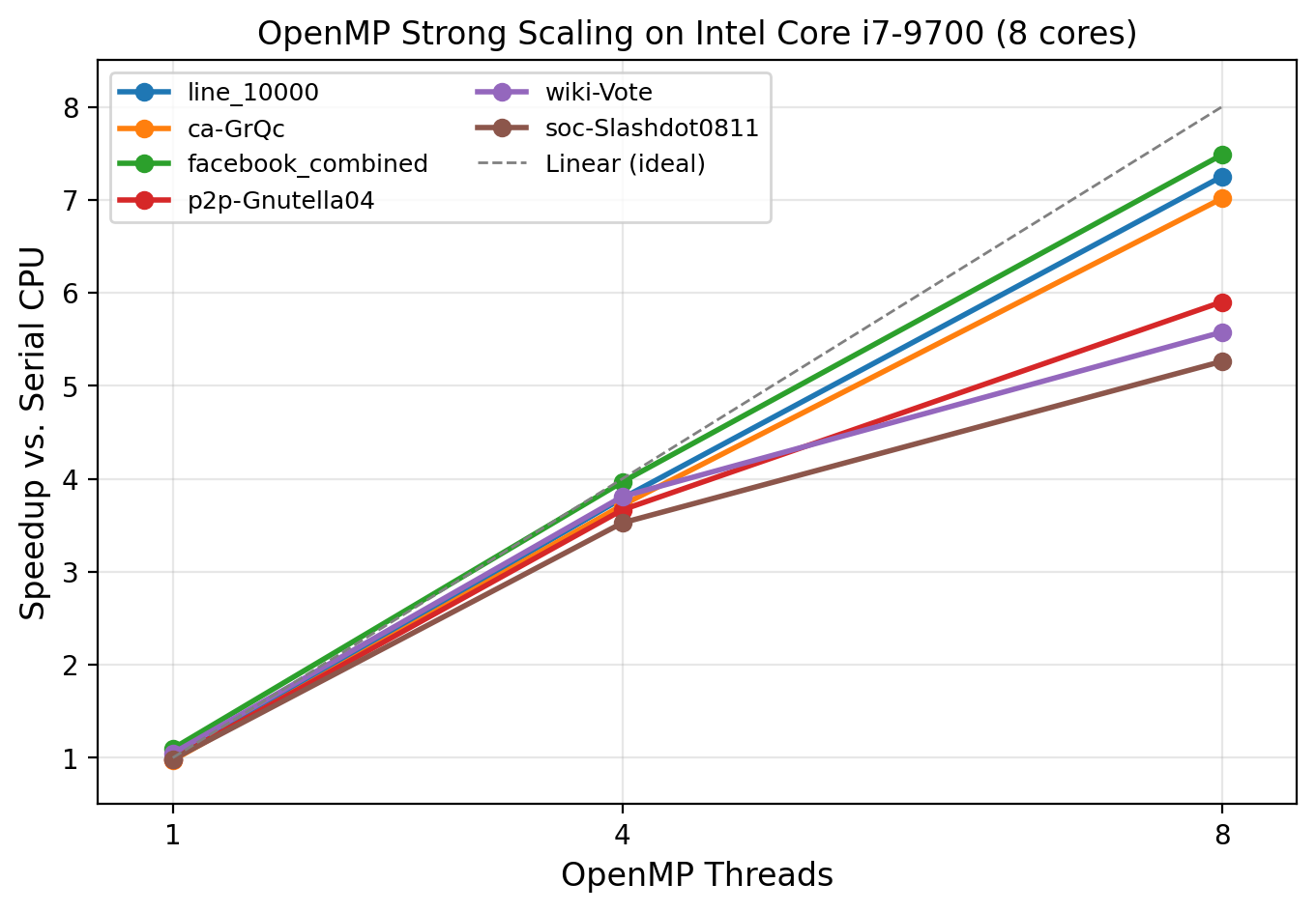
The OpenMP implementation scales near-linearly on regular and
sparse graphs and plateaus at 5-5.5× on the larger or more
skewed ones. line_10000 and ca-GrQc
reach over 7× at 8 threads. wiki-Vote and
soc-Slashdot0811 cap closer to 5.3× because
of degree skew and L3 cache pressure. ego-facebook
is dense but small enough to fit in L3, so it scales as well as
the sparse graphs.
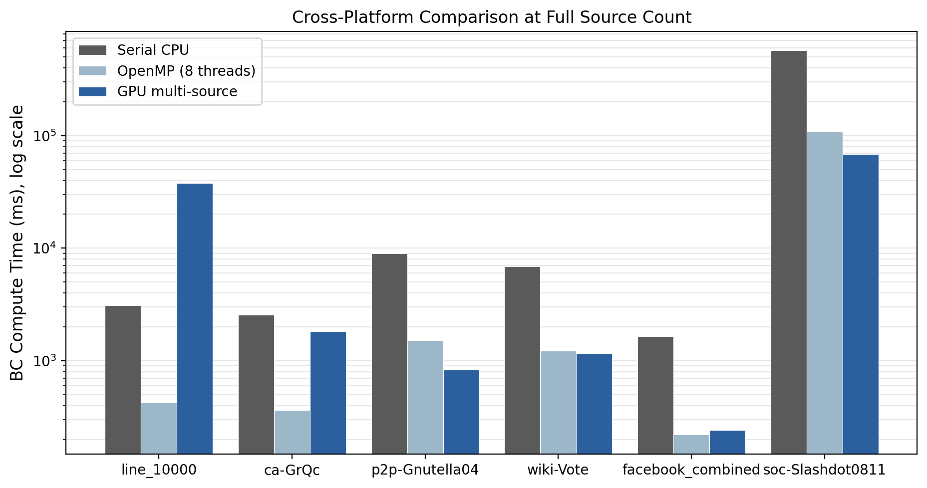
Cross-Platform Comparison at Full Source Count
The two parallel tracks tell different stories on different
graphs. The GPU multi-source design wins on graphs with enough
work per BFS to amortize per-chunk setup. OpenMP wins on graphs
small enough to fit in L3. The crossover is roughly the size of
p2p-Gnutella04.
The biggest GPU win is soc-Slashdot0811, where the
GPU finishes in 68 seconds versus 108 seconds at 8 threads on
the CPU and nearly 10 minutes on the serial baseline. On the
other end, ca-GrQc is small enough that the CPU is
5× faster than the GPU because the GPU spends most of its
time launching kernels and synchronizing source chunks.
Sampled BC at Large Scale
Sampled BC runtime is linear in the number of sampled sources
with per-source cost essentially flat between 67 and 72 ms on
web-Google. At 1,000 samples the BC compute time is
about 70 seconds. Exact all-source BC on the same graph would
require roughly 18 hours.
Accuracy was measured on ca-GrQc via top-k
overlap against the exact OpenMP ranking. With 1,000 samples,
the top-50 set matches the exact ranking at 82% overlap. More
samples give better agreement and the high-BC vertices stabilize
first.
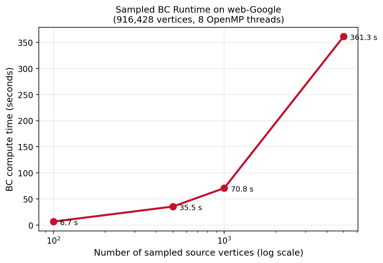
web-Google at 8
threads, log-x. Linear scaling with sample count.
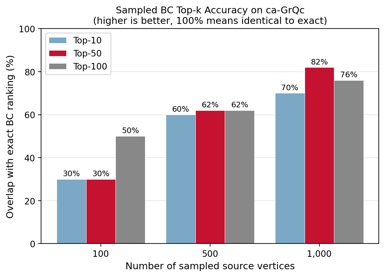
ca-GrQc, the top-50 matches
the exact ranking at 82% overlap.
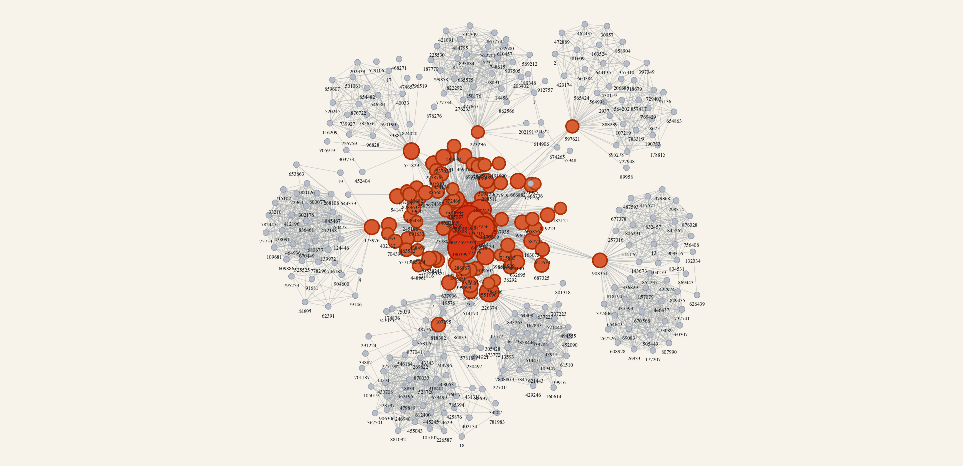
web-Google top-100 BC vertices recovered via the
sampled CPU mode.
What Limits Each Platform
CPU Limits at 8 Threads
-
Degree skew and load imbalance. Hub vertices
dominate BFS work for some sources, so threads with hub-heavy
assignments finish much later. Most visible on
wiki-Voteandsoc-Slashdot0811. - DRAM bandwidth. BFS and the dependency pass are pointer-chasing workloads that do little arithmetic per edge. Once cache misses land in DRAM, the implementation is memory-bandwidth-bound, not compute-bound.
-
L3 cache. Larger graphs do not fit.
ego-facebookis the exception that confirms the diagnosis, since it is dense but small enough to stay in L3 and so it scales as well as the sparse graphs.
GPU Limits
On graphs where the GPU wins, the constraint is hub-vertex
memory contention. The multi-source design fixed the
SM-utilization and host-sync bottlenecks, but per-vertex
atomicAdd on path counts and dependencies is
unchanged. On dense social graphs warps still spend many cycles
waiting on global memory at high-degree vertices.
Conclusion
The right target machine depends on the graph. For social and
web-scale graphs, the GPU was the right choice. The 1.58×
improvement over 8-thread OpenMP on
soc-Slashdot0811, on top of the 5.35× OpenMP
speedup over serial, amounts to an 8.3× end-to-end
improvement over the serial baseline on a representative
real-world graph. For small graphs OpenMP is faster and the
GPU's overheads are too much. The practical answer is to pick
the platform by graph size at runtime, with small graphs going
to OpenMP and large graphs going to the GPU.
The sampled CPU mode extends the same approach to graphs where
even 8 threads of exact Brandes is impractical, recovering the
high-BC ranking on web-Google in 70 seconds where
exact BC would take hours.
Work Distribution
50% / 50% split.
Yi-Ning Huang
- Implemented multi-core CPU code (serial baseline and OpenMP parallel version).
- Implemented sampled-source BC for large scale graphs and ran the runtime and accuracy experiments.
- Built the shared CSR graph loader, benchmark harness, and dataset pipeline.
- Ran all CPU benchmarks and produced the OpenMP scaling and dataset visualization figures.
Isaiah Velez
- Implemented GPU code using CUDA, including the iteratively profiled optimization sequence (edge-parallel, vertex-parallel, batched levels, active-vertex queue, multi-source).
- Ran Nsight Compute and Nsight Systems profiling to identify the three GPU bottlenecks and verify each design's effect.
- Ran all GPU benchmarks and produced the GPU journey and cross-platform comparison figures.
- Set up the build system on the GHC machines and integrated the GPU path into the shared CLI and benchmark flow.